🧠 Deep Learning for Time Series Forecasting
Time series forecasting is critical in domains like finance, weather prediction, inventory management, and traffic analysis. Traditional statistical methods such as ARIMA and exponential smoothing have limitations in capturing complex patterns. In this tutorial, we dive deep into using deep learning techniques like LSTM, GRU, and CNN for sequence modeling.

📘 What is Time Series Forecasting?
Time series forecasting is the process of using past observations to predict future values. The core idea is to model the sequence dependency of observations over time. Deep learning models like LSTM are designed for this purpose.
Click here for exclusive offer!- Stock price prediction
- Sales and demand forecasting
- Energy consumption prediction
- Temperature and weather modeling
- Patient monitoring in healthcare

🔍 Why Use Deep Learning?
Deep learning models like RNNs, LSTMs, and GRUs are capable of learning complex temporal dependencies that traditional models struggle with. They automatically extract features from sequential data, removing the need for manual feature engineering.
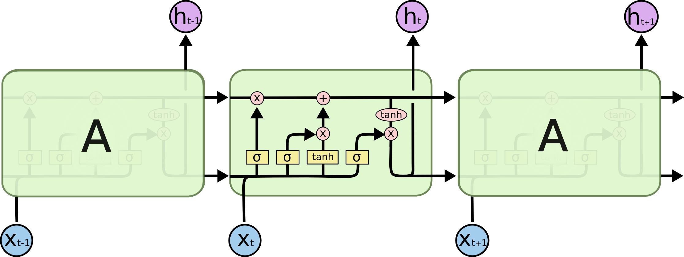
📚 LSTM – Long Short-Term Memory
LSTM networks are a type of recurrent neural network (RNN) that solve the vanishing gradient problem using memory cells. These cells can remember information for long durations, making LSTM ideal for time series tasks.

from tensorflow.keras.models import Sequential
from tensorflow.keras.layers import LSTM, Dense

model = Sequential()
model.add(LSTM(50, return_sequences=False, input_shape=(10, 1)))
model.add(Dense(1))
model.compile(optimizer='adam', loss='mse')
model.fit(X_train, y_train, epochs=20, batch_size=16)
⚙️ GRU – Gated Recurrent Unit
GRUs simplify the LSTM architecture by combining the forget and input gates into a single update gate. They are faster and perform comparably well for many tasks.
from tensorflow.keras.layers import GRU

model = Sequential()
model.add(GRU(64, input_shape=(30, 1)))
model.add(Dense(1))
model.compile(optimizer='adam', loss='mse')
model.fit(X_train, y_train, epochs=15)
🌀 Using 1D CNNs for Time Series
Convolutional Neural Networks (CNNs) can also be used for time series forecasting by treating the time dimension as spatial. 1D convolutions extract useful patterns from short windows of time.
📐 Data Preparation Tips
- Normalize the data using MinMaxScaler or StandardScaler.
- Reshape input into 3D format for LSTM/GRU:
(samples, timesteps, features). - Create sequences using sliding windows.
💡 Evaluation Metrics
- Mean Squared Error (MSE)
- Mean Absolute Error (MAE)
- Root Mean Squared Error (RMSE)
📁 Real-World Case Study: Forecasting Energy Consumption
Let’s apply LSTM to forecast hourly electricity consumption using an open dataset like the UCI Household Power Consumption dataset.
- Load and clean the dataset.
- Resample to hourly averages.
- Normalize values using MinMaxScaler.
- Create input/output sequences (X, y).
- Train/test split.
- Build LSTM model and train.
- Evaluate and plot predictions.
📈 Visualizing Forecasts
Use Matplotlib to plot the predicted vs actual values. It helps visually validate the model’s performance.
import matplotlib.pyplot as plt
plt.plot(y_test, label='Actual')
plt.plot(predictions, label='Predicted')
plt.legend()
plt.show()
📊 Performance Comparison
| Model | RMSE | Training Time |
|---|---|---|
| LSTM | 0.025 | 45s |
| GRU | 0.026 | 30s |
| 1D CNN | 0.029 | 20s |
🧠 Tips for Better Accuracy
- Use dropout layers to reduce overfitting.
- Experiment with different window sizes and batch sizes.
- Try hybrid models like CNN-LSTM for best results.
✅ Summary
- Deep learning provides flexible tools for sequence modeling.
- LSTM and GRU are powerful for capturing temporal dependencies.
- Proper data preparation is critical for good forecasting.
- Experimentation is key—try various architectures!
Comments
Post a Comment